Geoprocessing Services

Introduction:

In the world of GIS data is very valuable but being able to manipulate that data in a way that allows for analysis to take place is what makes GIS powerful.  This is done using geoprocessing.  This lab is designed to create a geoprocessing service and then incorporate that into a webmap.  A geoprocessing model will be created that solves multiple tasks, a geoprocessing service will be authored and published, and a Web GIS geoprocessing widget will be created to facilitate consuming that geoprocessing service.  In this lab, a mock business scenario is used as the objective of the geoprocessing service.   TFC Manufacturers is looking for a new area to put factories and needs to narrow their search area down based on a few criteria.  The locations must be close to a river, and a railroad as well as in close proximity to a city will a population greater than 4000.  The geoprocessing service created in this lab will allow the user to drop a point and it will show them the areas near that point that meet all of the criteria.

Methods:

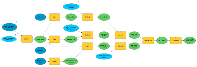
The first step to this lab was to create a model in ArcMap that the geoprocessing service will be based on.  Figure 1 below shows the model that the geoprocessing service is based on.  This model was created by adding features (Rivers, Railroads, Wisconsin_Cities) and tools.  These tools were connected to the features and outputs.  The model begins by clipping the river and railroad classes based on the buffer from the point class the user added to the map.  These clips are then buffered based on a distance that the user inputs (default 5 km),  these buffers are then intersected into a River_Rail_Int output.  The Wisconsin_Cities class is first ran through a select tool that selects all the cities with a population greater than 4000.  These cities are then clipped based on the point buffer class that the user inputted.  These cities are now joined to the river and rail intersect class based on a spatial join.  Finally these classes are all dissolved and a single polygon class is the final output (Factory_OptimalLocation) that shows the optimal area for a factory in that area.  The proper classes were then set as parameters by right clicking and selecting model parameter.  This makes these inputs that the user can change when they use the model as a geoprocessing service. These parameters can be seen in the model by the P next to them.   

Figure 1: Model

After the model was created, it was time to publish the model as a geoprocessing service.  This was done by running the model then selecting it in the results windows and clicking Share As- Geoprocessing Service.  When publishing the service, the execution mode was set to asynchronous, the parameters were given descriptions, the map was given an item discription and the geoprocessing service was published.

The next step is to create a web map using the developer edition of the Web App Builder.  A simple web application is created and the geoprocessing widget is brought in.  The geoprocessing widget is then given the service created in ArcMap.  This is done by referencing the service url in the server it was published to.  The map name and other descriptions were changed to make the map more user friendly.  Once this was done the app was ready to be moved to the development server.  This was done by downloading the map and extracting it into the server.   


Results:

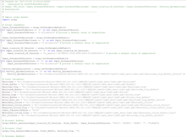
The model created above is a easy way to "write code."  The following image is python code that was created from the model.  It creates variables, sets parameters and determines when to run them.  This could be done by hand ArcMap provides the model builder for an easier more interactive way to do this.  This is the script that is behind the geoprocessing service that is added to the webmap.

Figure 2: Python Code from Model 1

Figure 3: Python Code from Model 2

The developer edition of the Web App Builder was used to create the following web application.  It is a simple ESRI template but gives the user (TFC Manufacturing) what they need.  The user simply has to click on the geoprocessing widget in the top left corner under the search bar to access the geoprocessing tool.   

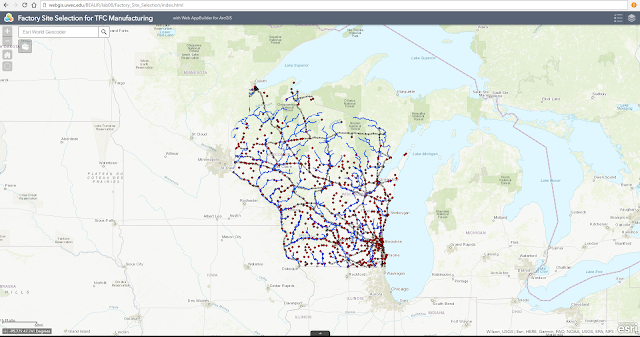
Figure 4: Final Map

The user is then given the opportunity to change the parameters of the tool and select a point of interest.  The user simply clicks the location of interest button and then selects a location on the map.  They then scroll down on the tool and select the execute button. 

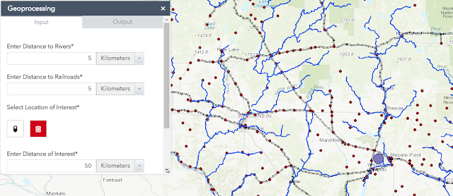
Figure 5: User Input

The geoprocessing tool then outputs the areas that meet all the criteria that were input above.  This output is given as a polygon.  The user can the hit the X on the geoprocessing panel to repeat the process with a different location.  This map could be optimized by allowing the user to save their outputs to be referenced at a later date.   

Figure 6: Output

Geoprocessing is an area of GIS that makes it so appealing to government agencies and private companies.  This relatively simple geoprocessing tool can make a multi-million dollar decision that much easier.  It also creates a visual representation of a phenomenon that would be hard to explain in words.  WebGIS has made it easy to give these tools to people who have no GIS experience.   Maps are a powerful tool and geoprocessing makes them even more powerful.

Sources:

Cyril Wilson